Why d log T Particles Are Enough, and What Carries Over to Networks
Exploration at Scale, Part 2: the cloud as a random projection, a Johnson–Lindenstrauss lemma for adaptive data, and the same update as an SGD step
Exploration at Scale · Part 2 of 2. Part 1 built Thompson sampling from a cloud of M particles and a random index. Based on Ensemble++ (NeurIPS 2025), HyperAgent (ICML 2024) and Probability Tools for Sequential Random Projection.
- The particles are a random projection of the data history, so tracking the posterior is a Johnson–Lindenstrauss statement.
- When the agent picks its own data, the noise reaches the inputs and the classical lemma no longer applies.
- A sequential Johnson–Lindenstrauss lemma survives adaptivity at the price of one log T, so d log T particles match Thompson sampling, against (actions × T) before.
- In a network the same update is an SGD step on M linear heads: architecture and optimizer designed together.
The figures step through like slides. Use → or ▶, and step back with ←.
1. The particles are a random projection of the history
Each particle is the whole data history weighted by one random direction, so M particles are M random projections of it.
So the injected noise is a Johnson–Lindenstrauss projection of the history, maintained as a stream. How small can M be?
Write the history as $\Phi_t$ (the prior, then one column per input) and the injected noise as $\Pi_t$ (the prior draws, then one row per data point). The arrows of the cloud are their product, and its covariance is
$$ \mathbf{A}_t = \Sigma_t\,\Phi_t\,\Pi_t, \qquad \mathbf{A}_t\mathbf{A}_t^{\top} = \Sigma_t\,\Phi_t\big(\Pi_t\Pi_t^{\top}\big)\Phi_t^{\top}\,\Sigma_t \;=\; \Sigma_t \quad\text{if } \Pi_t \text{ preserves norms on the history.} $$A new data point appends one column and one row, so the product changes by a rank-one term and never grows. The injected noise is a Johnson–Lindenstrauss projection of the history from $d+t$ dimensions down to M, maintained as a stream.
2. Once the agent picks its own data, the classical lemma fails
The noise is drawn once and never redrawn, which keeps the update cheap, but it also means the old noise steers the inputs the agent chooses next.
data
particle
injected noise
Thin arrows: the update
Thick arrows: the particle picks the next input
Fixed data
- inputs fixed in advance
- injected noise never reaches them
- classical JL applies
Adaptive data
- each particle picks the next input
- old injected noise steers the history
- classical JL fails
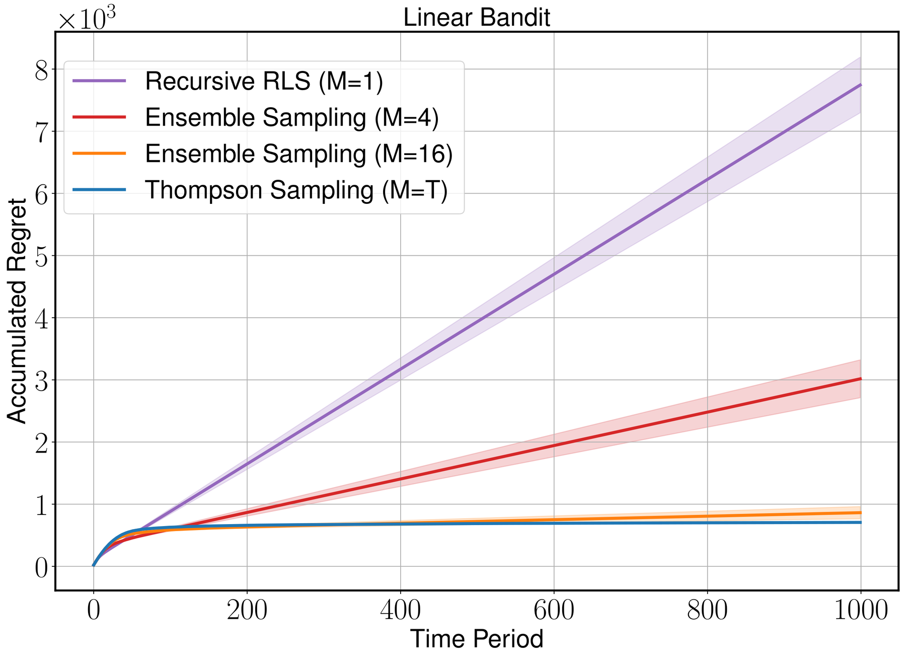
One particle (M = 1): regret grows linearly. Thompson sampling flattens.
With fixed data the classical lemma applies; with adaptive data it does not. With one particle the regret grows linearly, while Thompson sampling flattens.
The classical lemma needs the vectors to be fixed before the projection is drawn. Here each new column of the history is chosen after the agent has seen earlier rows of the noise. That dependence is also why the only earlier analysis (Qin et al., 2022) needed an ensemble linear in the horizon times the number of actions. Practitioners had been using 10 to 100 members for a decade without an explanation.
3. Sequential Johnson–Lindenstrauss: adaptivity costs one log T
Norms are preserved for adaptively chosen sequences, uniformly over time, with one extra logarithm of the horizon.
Let $\mathbf{z}_i$ be the rows of the injected noise and $v$ a vector of the history whose entries may depend on all earlier rows. Then, with probability at least $1-\delta$,
$$ M \ge \frac{C}{\varepsilon^2}\Big(\log\frac1\delta + \log T\Big) \;\Longrightarrow\; \forall\, t \le T:\quad (1-\varepsilon)\sum_{i\le t} v_i^2 \;\le\; \Big\|\sum_{i\le t} v_i\,\mathbf{z}_i\Big\|^2 \;\le\; (1+\varepsilon)\sum_{i\le t} v_i^2 . $$Independence cannot be used, so the proof runs through a stopped process and self-normalized martingale concentration. For the cloud, the result reads
$$ M \ge C\,d\log T \;\Longrightarrow\; \tfrac12\,\Sigma_t \preceq \mathbf{A}_t\mathbf{A}_t^{\top} \preceq \tfrac32\,\Sigma_t \qquad \forall\, t \le T . $$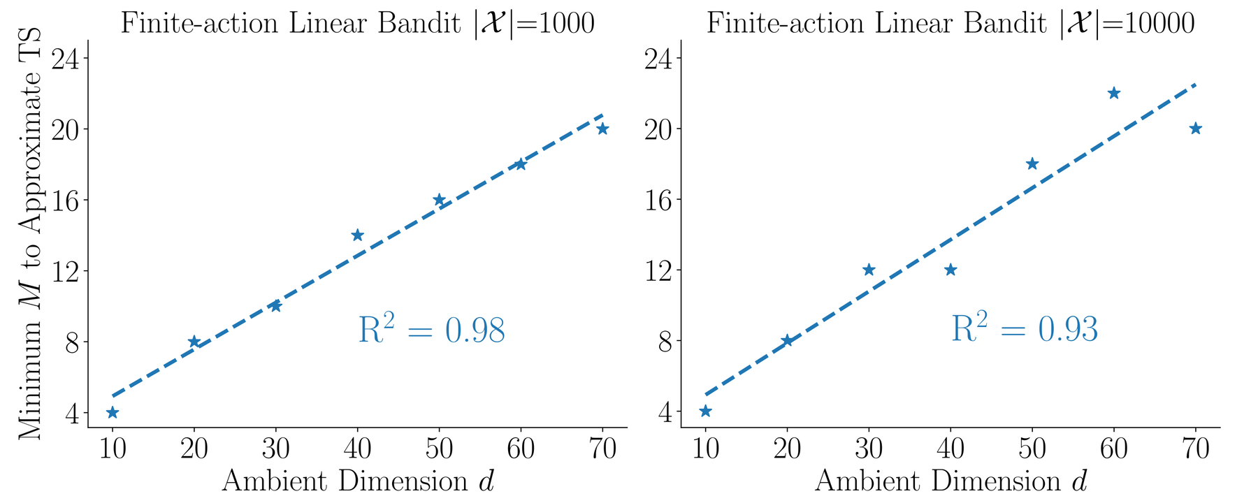
With M of order d log T, the regret is comparable to exact Thompson sampling for compact or finite action sets, fixed or time-varying. Memory grows with the logarithm of the lifetime: doubling the horizon adds a number of particles proportional to d, however long the agent has already run.
4. In a network the same update is an SGD step
The exact gain of the linear model becomes a learning rate, and each particle becomes a linear head trained on its own noisy targets.
Nothing in the training loop changes except the targets.
The posterior sampler is trained by the same stochastic updates as the model, on the same data stream, at the cost of a few extra linear heads. Seen from the network’s side, the model has a second input:
HyperDQN (ICLR 2022), HyperAgent (ICML 2024) and Ensemble++ (NeurIPS 2025) cover the three levels.
Neither half works alone. Without the noisy targets, a network learns to ignore the index. Without the index, the noisy targets give one perturbed model, and the next sample needs a full retraining.
| Architecture | Optimization | |
|---|---|---|
| Design | A second input, the random index; output linear in it (a mean head plus M index heads), each with a fixed random prior | Every head’s target carries its own injected noise, drawn once per data point; minibatch SGD from a bounded FIFO buffer |
| Cost | Memory: M extra linear heads and a bounded buffer, no covariance matrix | Step: a fixed number of SGD steps per interaction. Sample: one forward pass with a fresh index |
Where the index should enter (the last layer, deeper layers, adapters on a large model) is a design choice that is still largely unexplored.
5. Results: less data, fewer parameters
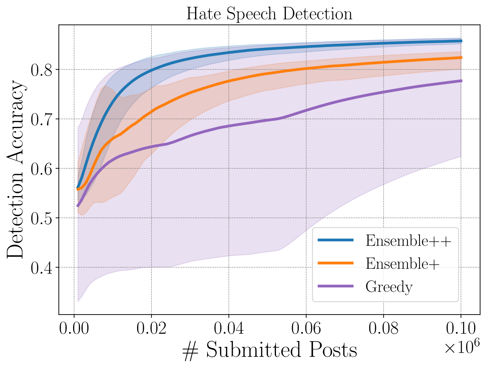
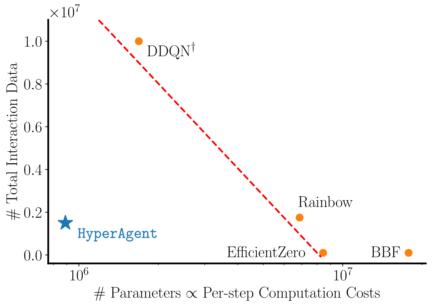
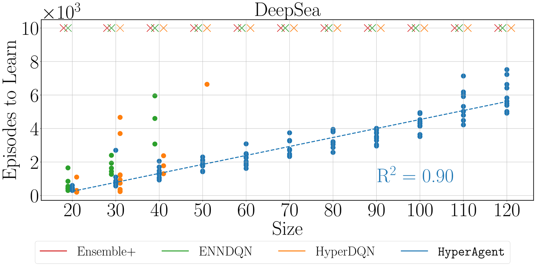
Directed exploration buys the data efficiency, and a few linear heads keep the compute bounded.
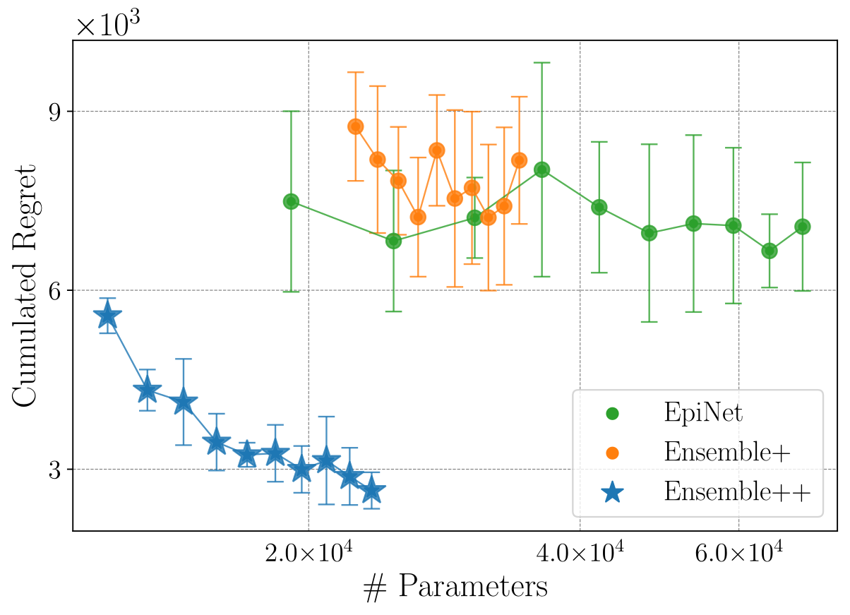
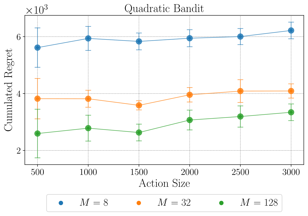
In deep RL, HyperAgent adds the same heads to DQN:
References
- Y. Li, J. Xu, B. Wang, Z.-Q. Luo. Scalable Exploration via Ensemble++. NeurIPS 2025.
- Y. Li, J. Xu, L. Han, Z.-Q. Luo. Q-Star Meets Scalable Posterior Sampling: Bridging Theory and Practice via HyperAgent. ICML 2024.
- Y. Li. Probability Tools for Sequential Random Projection. arXiv, 2024.
- Z. Li, Y. Li, Y. Zhang, T. Zhang, Z.-Q. Luo. HyperDQN: A Randomized Exploration Method for Deep Reinforcement Learning. ICLR 2022.
- C. Qin, Z. Wen, X. Lu, B. Van Roy. An Analysis of Ensemble Sampling. NeurIPS 2022.
Citation
@inproceedings{li2024hyperagent,
  title     = {Q-Star Meets Scalable Posterior Sampling: Bridging Theory and Practice via HyperAgent},
  author    = {Li, Yingru and Xu, Jiawei and Han, Lei and Luo, Zhi-Quan},
  booktitle = {International Conference on Machine Learning},
  year      = {2024}
}

Yingru Li
Member of Technical Staff
Core contributor to RL fundamentals at xAI (now SpaceX Super Intelligence); I make reinforcement learning on frontier models stable, efficient, and scalable.