Information Bandwidth in Reinforcement Learning
How Gradient Structure Determines Information Capacity
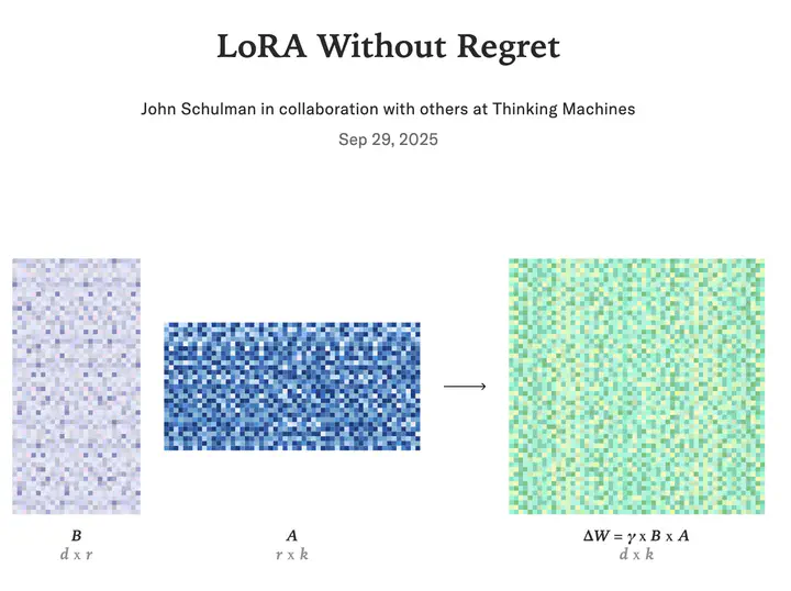 “LoRA without Regret”
How Gradient Structure Determines Information Capacity
When I first read the “LoRA Without Regret” blog post, one claim caught my attention: policy gradient algorithms learn roughly 1 bit of information per episode. This insight elegantly explains why LoRA—with its mere thousands of trainable parameters—works so remarkably well for RL fine-tuning of large language models.
But what does this actually mean? The key insight is that this 1-bit limit applies specifically to scalar advantage formulations—where all rewards are aggregated into a single number. In this post, I’ll show that the information ceiling depends critically on gradient structure: scalar advantage (≤ log₂(B) bits) versus per-timestep advantages (≤ H(r) bits).
TL;DR: The Main Results
Scalar advantage formulation: When the gradient uses a single scalar advantage aggregating all rewards—$g = \nabla \log p_\theta(\tau) \cdot \text{Adv}$ where $\text{Adv} = G - b$—the information ceiling is $\leq \log_2(B)$ bits per episode. Given the training history, the direction term $\nabla \log p_\theta(\tau)$ is independent of rewards; only the scalar advantage carries reward information. For binary feedback, this is $\leq 1$ bit/episode.
Per-timestep advantage formulation: When the gradient uses advantages at each timestep—$g = \sum_t \nabla \log \pi_\theta(a_t|s_t) \cdot A_t$—the information ceiling equals the reward entropy: $I(g; \pi^\star \mid \mathcal{H}) \leq H(\mathbf{r} \mid \tau, \mathcal{H})$. This applies to both:
- REINFORCE with returns: $A_t = G_t - b$ where $G_t = \sum_{k \geq t} \gamma^{k-t} r_k$
- Actor-critic with TD errors: $A_t = \delta_t = r_t + \gamma V_\phi(s_{t+1}) - V_\phi(s_t)$
Both preserve information because the mappings ${A_t} \leftrightarrow {\mathbf{r}}$ are bijective.
Reward structure determines the gap:
- Terminal rewards only: $H(\mathbf{r}) \leq 1$ bit → all formulations achieve ≤ 1 bit
- Dense independent rewards ($T=1000$, ternary): $H(\mathbf{r}) \approx 1585$ bits → scalar achieves ≤ 8 bits, per-timestep achieves ≤ 1585 bits
| Gradient Formulation | Terminal Reward | Dense Independent Rewards | Asymptotic (Dense) |
|---|---|---|---|
| Scalar advantage | ≤ 1 bit | ≤ 8 bits | $O(\log T)$* |
| Per-timestep advantages | ≤ 1 bit | ≤ 1585 bits | $O(T)$ |
*$O(\log T)$ without finite precision; saturates to $O(1)$ for large $T$ with finite precision
The remainder of this post derives these bounds rigorously.
Part 1: The Mathematical Framework
Setup: Language Model Fine-Tuning as an MDP
When you fine-tune an LLM with RL, you’re working with a special kind of problem:
- States $s$: Token sequences $(x_1, \ldots, x_t)$
- Actions $a$: Next token $x_{t+1}$ from vocabulary
- Transitions: Deterministic (append token: $s’ = s \circ a$)
- Rewards $R_\xi$: Determined by unknown parameter $\xi$ (preferences, objectives)
Key property: Transitions are known and deterministic. All uncertainty is in the reward function $\xi$.
Information-Theoretic Lens
To analyze this rigorously, we need a mathematical trick. Put a prior $p(\xi)$ over reward parameters—this induces a distribution $p(\pi^\star)$ over optimal policies, where each $\xi$ determines a unique optimal policy $\pi^\star_\xi$.
We don’t claim algorithms actually maintain Bayesian posteriors. This is just a modeling device that lets us reason about information flow: it makes both the learning signal (the gradient) and the optimal policy $\pi^\star$ well-defined random variables, so we can compute their mutual information.
Definition (Information Bandwidth):
The information bandwidth measures the maximum information that can be gained per episode:
$$\mathcal{B} = \sup_{\mathcal{H}} I(g; \pi^\star \mid \mathcal{H})$$
where $g$ is the gradient from a single episode and $\mathcal{H}$ is the history of all previous episodes.
Interpretation: $I(g; \pi^\star \mid \mathcal{H})$ asks “how much does this gradient tell me about the optimal policy, given what I already know?” The bandwidth $\mathcal{B}$ is the maximum—the algorithm’s capacity limit regardless of training progress. In practice, history gets compressed into parameters $\theta$, but conditioning on the complete history $\mathcal{H}$ makes the information-theoretic interpretation most transparent: it directly captures “what we’ve already learned” from all past episodes.
Connection to the Original Insight
This formalization directly implements the information-theoretic argument from “LoRA Without Regret.” Their key observation: for the scalar-advantage REINFORCE gradient $g = \nabla \log p_\theta(\tau) \cdot \text{Adv}$, the component $\nabla \log p_\theta(\tau)$ is independent of the reward function $R$ given the history $\mathcal{H}$ (which determines the policy), so all information about $R$ must flow through the scalar advantage.
We extend this by analyzing how different gradient structures preserve or destroy information.
Two Minimal Assumptions
Assumption A1 (Unique Optimum): Each $\xi$ determines a unique optimal policy $\pi^\star_\xi$.
Justification: Generic for neural networks with many parameters. Floating-point precision breaks ties; exact degeneracy is measure-zero.
Assumption A2 (Finite Resolution): The reward-dependent scalar(s) in the gradient have finite effective resolution—they can take at most $B$ distinguishable values.
Justification: Holds exactly for binary preferences ($B=2$) or Likert scales ($B=4$-$7$). Approximately true for continuous signals with noise, finite precision, or practical distinguishability limits.
Note on asymptotic behavior: For scalar advantages with dense rewards, $B$ effectively equals $\min(2T+1, B_{\text{max}})$ where $B_{\text{max}}$ is the precision limit. This gives $O(\log T)$ bits for small $T$ and $O(1)$ bits for large $T \gg B_{\text{max}}$. Examples below use large $T$ where saturation applies.
Part 2: Scalar Advantage Information Ceiling
The Scalar Advantage Formulation
The standard scalar-advantage REINFORCE algorithm works like this:
- Sample trajectory $\tau = (s_0, a_0, \ldots, s_{T-1}, a_{T-1}, s_T)$ using policy $\pi_\theta$
- Observe rewards $\mathbf{r} = (r_0, r_1, \ldots, r_{T-1})$ where $r_t = R_\xi(s_t, a_t)$
- Compute return: $G = \sum_{t=0}^{T-1} \gamma^t r_t$
- Compute advantage: $\text{Adv} = G - b$ (where $b$ is a baseline)
- Compute gradient: $g = \nabla \log p_\theta(\tau) \cdot \text{Adv}$
- Update: $\theta \leftarrow \theta + \alpha g$
Key observation: The gradient has two components:
- $\nabla \log p_\theta(\tau)$: Independent of the reward function $R$ given the history $\mathcal{H}$
- $\text{Adv}$: A scalar that encodes all reward-dependent information
The Information Ceiling
Theorem 1 (Scalar Advantage Information Ceiling):
Under assumptions A1 and A2, the information bandwidth of scalar-advantage formulations satisfies:
$$I(g; \pi^\star \mid \mathcal{H}) \leq \log_2(B) \text{ bits per episode}$$
where $g = \nabla \log p_\theta(\tau) \cdot \text{Adv}$ with $\text{Adv} = G - b$ is the gradient and $\mathcal{H}$ is the history of all previous episodes.
Intuition: Given the history $\mathcal{H}$ (which determines the current policy $\theta$), the trajectory sampling doesn’t depend on $\xi$. All new information must flow through the scalar advantage, creating a hard ceiling of $\log_2(B)$ bits.
Asymptotic interpretation: For dense rewards without Assumption A2, the return can take up to $2T+1$ values, giving $O(\log T)$ bits. With finite precision $B_{\text{max}}$, the bound becomes $O(\min(\log T, \log B_{\text{max}}))$. For typical LLM fine-tuning with large $T \gg B_{\text{max}}$, this saturates at $O(1)$ bits.
Detailed Proof (click to expand)
Step 1: Information Chain
By data processing inequality, since $g$ is a deterministic function of $(\tau, \text{Adv})$ given $\mathcal{H}$: $$I(g; \pi^\star \mid \mathcal{H}) \leq I((\tau, \text{Adv}); \pi^\star \mid \mathcal{H})$$
By chain rule for mutual information: $$I((\tau, \text{Adv}); \pi^\star \mid \mathcal{H}) = I(\tau; \pi^\star \mid \mathcal{H}) + I(\text{Adv}; \pi^\star \mid \tau, \mathcal{H})$$
Step 2: Trajectory Contains No Information About $\xi$
Given $\mathcal{H}$, the policy parameters $\theta = \theta(\mathcal{H})$ are deterministic. The trajectory is sampled from: $$\tau \sim p_\theta(\tau)$$
This distribution depends only on $\theta$ (and the known, deterministic environment dynamics), not on the reward parameter $\xi$.
Therefore: $\tau \perp \xi \mid \mathcal{H}$
Since $\xi$ determines $\pi^\star$ deterministically by Assumption A1, we also have $\tau \perp \pi^\star \mid \mathcal{H}$.
Therefore: $$I(\tau; \pi^\star \mid \mathcal{H}) = 0$$
Step 3: All Information Flows Through Advantage
From Steps 1-2: $$I(g; \pi^\star \mid \mathcal{H}) \leq I(\text{Adv}; \pi^\star \mid \tau, \mathcal{H})$$
Step 4: Bound Advantage Information
By the fundamental bound on mutual information: $$I(\text{Adv}; \pi^\star \mid \tau, \mathcal{H}) \leq H(\text{Adv} \mid \tau, \mathcal{H})$$
Step 5: Apply Finite Resolution Assumption
By Assumption A2, the advantage takes at most $B$ distinct values. Therefore: $$H(\text{Adv} \mid \tau, \mathcal{H}) \leq \log_2(B)$$
This holds because entropy is maximized when uniform: $H(X) \leq \log_2(|X|)$
Final Result
Combining all steps: $$I(g; \pi^\star \mid \mathcal{H}) \leq I(\text{Adv}; \pi^\star \mid \tau, \mathcal{H}) \leq H(\text{Adv} \mid \tau, \mathcal{H}) \leq \log_2(B)$$
∎
This ceiling holds regardless of sequence length $T$, model size, or computational budget—it’s an inherent consequence of the scalar advantage bottleneck.
Where Does Information Get Lost?
The bound $\leq \log_2(B)$ is tight for some reward structures but loose for others:
$$\mathbf{r} \xrightarrow{\text{sum}} G \xrightarrow{\text{subtract baseline}} \text{Adv} \xrightarrow{\text{finite resolution}} \text{bounded by } B$$
Case 1: Terminal Reward Only
Setup: $r_t = 0$ for $t < T-1$, only $r_{T-1} \in \{-1, +1\}$ is non-zero
Return: $G = \gamma^{T-1} r_{T-1}$
Advantage: $\text{Adv} = \gamma^{T-1} r_{T-1} - b$
Since the mapping $r_{T-1} \leftrightarrow \text{Adv}$ is bijective: $$H(\text{Adv} \mid \tau, \mathcal{H}) = H(r_{T-1} \mid \tau, \mathcal{H}) = 1 \text{ bit}$$
No information loss from aggregation. The bound is tight.
Case 2: Dense Independent Rewards
Setup: $r_t \in \{-1, 0, +1\}$ at each timestep, with factorized $\xi = (\xi_0, \xi_1, \ldots, \xi_{T-1})$ where each $\xi_t$ is independent
Available information: $$H(\mathbf{r} \mid \tau, \mathcal{H}) = \sum_{t=0}^{T-1} H(r_t \mid \tau, \mathcal{H}) = T \log_2(3) \approx 1.58T \text{ bits}$$
For $T = 1000$: approximately 1585 bits available.
Return: $G = \sum_{t=0}^{T-1} \gamma^t r_t$
This is a many-to-one mapping. Different temporal patterns give the same sum:
- $(+1, -1, +1, -1, \ldots)$ → sum ≈ 0
- $(-1, +1, -1, +1, \ldots)$ → sum ≈ 0
- $(0, 0, 0, \ldots, 0)$ → sum = 0
For $\gamma = 1$, the return $G \in \{-1000, -999, \ldots, 999, 1000\}$ has: $$H(G \mid \tau, \mathcal{H}) \leq \log_2(2001) \approx 11 \text{ bits}$$
This is the $O(\log T)$ regime before finite precision effects.
Advantage: With noise and finite precision (Assumption A2 with $B = 256$): $$H(\text{Adv} \mid \tau, \mathcal{H}) \leq \log_2(256) = 8 \text{ bits}$$
Since $2001 > 256$, the advantage saturates at the precision limit—the $O(1)$ regime for large $T$.
Information loss: Starting with 1585 bits, the scalar advantage retains only ~8 bits.
Loss factor: ~200× reduction
Why? The summation loses temporal structure. Different temporal reward patterns can produce the same scalar advantage.
Concrete Examples
- Binary preferences ($B=2$): $\leq 1$ bit/episode
- Likert scale ($B=5$): $\leq 2.3$ bits/episode
- 8-bit resolution ($B=256$): $\leq 8$ bits/episode
The Bottleneck
A typical LLM generation has $T \sim 1000$ tokens. The scalar-advantage formulation compresses all this rich structure into one scalar that modulates a fixed direction $\nabla \log p_\theta(\tau)$.
The policy update $\Delta \theta = \alpha g$ happens in a high-dimensional space, but the information content of this update about the optimal policy is fundamentally limited by the scalar advantage. This structural bottleneck cannot be overcome by adding more parameters or computational resources.
Part 3: Per-Timestep Advantages Preserve Information
The Per-Timestep Formulation
Instead of aggregating all rewards into one scalar, we can use advantages at each timestep:
$$g = \sum_{t=0}^{T-1} \nabla \log \pi_\theta(a_t|s_t) \cdot A_t$$
where $A_t$ is an advantage for timestep $t$. This structure appears in two common algorithms:
REINFORCE with per-timestep returns: $$A_t = G_t - b$$ where $G_t = \sum_{k \geq t} \gamma^{k-t} r_k$ is the return from timestep $t$ onward, and $b$ is a constant baseline.
Actor-critic with TD errors: $$A_t = \delta_t = r_t + \gamma V_\phi(s_{t+1}) - V_\phi(s_t)$$ where $V_\phi$ is a learned value function.
Key property: Both formulations preserve temporal structure by using $T$ advantages instead of one scalar.
Why Per-Timestep Advantages Preserve Information
Scalar advantage aggregates all rewards into one number: $$\text{Adv} = \sum_{t=0}^{T-1} \gamma^t r_t - b$$
This is a many-to-one mapping: different temporal patterns can give the same advantage. For $T=1000$ tokens with $r_t \in \{-1, 0, +1\}$ :
- Total available information: $H(\mathbf{r}) = 1000 \times \log_2(3) \approx 1585$ bits
- After summation: $H(\text{Adv}) \leq 8$ bits
- Information lost: ~99%
Per-timestep returns ${G_t}$ preserve information through a bijective mapping: $$G_t = \sum_{k \geq t} \gamma^{k-t} r_k$$
Given ${G_t}$, we can recover rewards: $r_t = G_t - \gamma G_{t+1}$ (with $G_T = 0$). Therefore: $$H({G_t} \mid \tau, \mathcal{H}) = H(\mathbf{r} \mid \tau, \mathcal{H})$$
TD errors ${\delta_t}$ also preserve information: $$\delta_t = r_t + \gamma V_\phi(s_{t+1}) - V_\phi(s_t)$$
Given $(\tau, \mathcal{H})$, the value terms are deterministic, so $\delta_t = r_t + c_t$ where $c_t$ is known. This is an invertible affine transformation: $$\mathbf{r} = \boldsymbol{\delta} - \mathbf{c}$$
Therefore: $H(\boldsymbol{\delta} \mid \tau, \mathcal{H}) = H(\mathbf{r} \mid \tau, \mathcal{H})$
Key insight: Both ${G_t}$ and ${\delta_t}$ preserve all reward information—they just redistribute it temporally instead of collapsing it into one scalar.
The Information Ceiling
Theorem 2 (Per-Timestep Advantages Information Ceiling):
Under assumptions A1 and A2 (applied to rewards with resolution $B_r$), per-timestep advantage formulations satisfy:
$$I(g; \pi^\star \mid \mathcal{H}) \leq H(\mathbf{r} \mid \tau, \mathcal{H})$$
where $\mathbf{r} = (r_0, \ldots, r_{T-1})$ is the reward sequence.
This applies to both REINFORCE with ${G_t}$ and actor-critic with ${\delta_t}$.
Special cases:
Terminal reward only: $H(\mathbf{r} \mid \tau, \mathcal{H}) = H(r_{T-1} \mid \tau, \mathcal{H}) \leq \log_2(B_r)$
Independent rewards (factorized $\xi$): $H(\mathbf{r} \mid \tau, \mathcal{H}) = \sum_t H(r_t \mid \tau, \mathcal{H}) \leq T \log_2(B_r)$
General case: $\log_2(B_r) \leq H(\mathbf{r} \mid \tau, \mathcal{H}) \leq T \log_2(B_r)$
Key insight: The ceiling depends on reward entropy, not on the specific form of advantages. Both ${G_t}$ and ${\delta_t}$ preserve the same amount of information.
Complete Rigorous Proof (click to expand)
Step 1: From Gradient to Advantages
The gradient is: $$g = \sum_{t=0}^{T-1} \nabla \log \pi_\theta(a_t|s_t) \cdot A_t$$
where $\mathbf{A} = (A_0, \ldots, A_{T-1})$ is either ${G_t - b}$ or ${\delta_t}$.
Given $(\tau, \mathcal{H})$:
- The policy $\theta = \theta(\mathcal{H})$ is deterministic
- All states and actions in $\tau$ are known
- The gradient is a deterministic function of $(\tau, \mathbf{A}, \mathcal{H})$
By data processing: $$I(g; \pi^\star \mid \mathcal{H}) \leq I((\tau, \mathbf{A}); \pi^\star \mid \mathcal{H})$$
By chain rule: $$I((\tau, \mathbf{A}); \pi^\star \mid \mathcal{H}) = I(\tau; \pi^\star \mid \mathcal{H}) + I(\mathbf{A}; \pi^\star \mid \tau, \mathcal{H})$$
Since $\tau \perp \xi \mid \mathcal{H}$: $$I(\tau; \pi^\star \mid \mathcal{H}) = 0$$
Therefore: $$I(g; \pi^\star \mid \mathcal{H}) \leq I(\mathbf{A}; \pi^\star \mid \tau, \mathcal{H})$$
Step 2: From Advantages to Rewards (The Key Step)
Case 1: Returns $A_t = G_t - b$
The returns satisfy: $$G_t = \sum_{k \geq t} \gamma^{k-t} r_k$$
This is invertible: $r_t = G_t - \gamma G_{t+1}$ (with $G_T = 0$).
Subtracting constant $b$ doesn’t change entropy: $$H({G_t - b} \mid \tau, \mathcal{H}) = H({G_t} \mid \tau, \mathcal{H}) = H(\mathbf{r} \mid \tau, \mathcal{H})$$
Case 2: TD errors $A_t = \delta_t$
Given $(\tau, \mathcal{H})$, the value function parameters $\phi = \phi(\mathcal{H})$ are deterministic, so: $$\delta_t = r_t + c_t$$ where $c_t = \gamma V_\phi(s_{t+1}) - V_\phi(s_t)$ is deterministic.
This is an affine transformation: $\boldsymbol{\delta} = \mathbf{r} + \mathbf{c}$, which is invertible.
Therefore: $$H(\boldsymbol{\delta} \mid \tau, \mathcal{H}) = H(\mathbf{r} \mid \tau, \mathcal{H})$$
Both cases: The mapping $\mathbf{A} \leftrightarrow \mathbf{r}$ is bijective, so: $$I(\mathbf{A}; \pi^\star \mid \tau, \mathcal{H}) = I(\mathbf{r}; \pi^\star \mid \tau, \mathcal{H})$$
Step 3: From Rewards to $\xi$
By Assumption A1, $\pi^\star = f(\xi)$ deterministically: $$\mathbf{r} \to \xi \to \pi^\star$$
By data processing: $$I(\mathbf{r}; \pi^\star \mid \tau, \mathcal{H}) \leq H(\mathbf{r} \mid \tau, \mathcal{H})$$
Final Result
Combining Steps 1-3: $$I(g; \pi^\star \mid \mathcal{H}) \leq H(\mathbf{r} \mid \tau, \mathcal{H})$$
∎
Analyzing the Reward Entropy
The bound $H(\mathbf{r} \mid \tau, \mathcal{H})$ depends on the structure of the reward function $R_\xi$.
Using the chain rule: $$H(\mathbf{r} \mid \tau, \mathcal{H}) = \sum_{t=0}^{T-1} H(r_t \mid r_{<t}, \tau, \mathcal{H})$$
where $r_{<t} = (r_0, \ldots, r_{t-1})$.
Each term satisfies: $$H(r_t \mid r_{<t}, \tau, \mathcal{H}) \leq \log_2(B_r)$$
The sum satisfies: $$H(\mathbf{r} \mid \tau, \mathcal{H}) \leq T \log_2(B_r)$$
Equality holds if and only if rewards are informationally independent: $r_t \perp r_{<t} \mid (\tau, \mathcal{H})$ for all $t$.
This requires factorized $\xi$: each state-action pair has its own independent reward parameter.
Case Analysis
Case 1: Terminal Reward Only
Setup: Only $r_{T-1} \neq 0$, all other rewards are zero
Reward entropy: $$H(\mathbf{r} \mid \tau, \mathcal{H}) = H(r_{T-1} \mid \tau, \mathcal{H}) \leq \log_2(B_r)$$
For binary rewards: $\leq 1$ bit
Per-timestep advantages: Whether using ${G_t - b}$ or ${\delta_t}$, only the terminal timestep carries information. All other advantages are deterministic given $(\tau, \mathcal{H})$.
Information ceiling: $I(g; \pi^\star \mid \mathcal{H}) \leq 1$ bit
Conclusion: Same as scalar advantage! When there’s only terminal reward, per-timestep formulations have no information advantage.
Case 2: Dense Independent Rewards
Setup: Factorized reward parameter $\xi = (\xi_0, \xi_1, \ldots, \xi_{T-1})$ where each $\xi_t$ is independent, and $r_t = R_{\xi_t}(s_t, a_t)$
This means: Observing $r_0$ reveals information about $\xi_0$ but nothing about $\xi_1, \ldots, \xi_{T-1}$.
Reward entropy: $$H(\mathbf{r} \mid \tau, \mathcal{H}) = \sum_{t=0}^{T-1} H(r_t \mid \tau, \mathcal{H}) = T \log_2(B_r)$$
Example ($T=1000$, $r_t \in \{-1, 0, +1\}$ so $B_r=3$): $$H(\mathbf{r} \mid \tau, \mathcal{H}) = 1000 \times \log_2(3) \approx 1585 \text{ bits}$$
Per-timestep advantages information ceiling: Up to 1585 bits/episode
Scalar advantage information ceiling: $\leq 8$ bits/episode
Advantage: $\sim 200\times$ more information preserved!
Why the difference?
- Scalar advantage: $\mathbf{r} \to \sum_t \gamma^t r_t$ loses temporal structure
- Per-timestep advantages: $\mathbf{r} \to {G_t}$ or $\mathbf{r} \to {\delta_t}$ preserves all information
Summary
| Gradient Formulation | Reward Structure | Information Ceiling | Asymptotic | Why |
|---|---|---|---|---|
| Scalar advantage | Terminal only | ≤ 1 bit | $O(1)$ | Single scalar with binary reward |
| Per-timestep advantages | Terminal only | ≤ 1 bit | $O(1)$ | Only one timestep is random |
| Scalar advantage | Dense independent | ≤ 8 bits | $O(\log T)$* | Aggregation loses temporal structure |
| Per-timestep advantages | Dense independent | ≤ 1585 bits | $O(T)$ | Temporal structure preserved |
*Saturates to $O(1)$ for large $T$ with finite precision
Part 4: Implications
The Core Insight
The information ceiling depends on two factors:
- Gradient structure: Scalar advantage (≤ log₂(B) bits, $O(\log T)$ asymptotically) vs per-timestep advantages (≤ H(r) bits, $O(T)$ asymptotically for dense independent rewards)
- Reward structure: Terminal (≤ log₂(B_r) bits, $O(1)$) vs dense independent (≤ T log₂(B_r) bits, $O(T)$)
Key observation: With terminal rewards only, scalar and per-timestep formulations have the same information ceiling (both $O(1)$ bits). This is why simple scalar-advantage methods dominate in LLM fine-tuning—the added complexity of per-timestep formulations provides no information-theoretic benefit when rewards are sparse.
When Structure Matters
Per-timestep advantages only help when rewards are dense and informative at each timestep. The potential gain scales with:
- Temporal density: How many timesteps provide informative rewards
- Independence: How much correlation exists between rewards at different timesteps
Asymptotic comparison:
- Dense independent rewards: $O(\log T)$ bits (scalar) vs $O(T)$ bits (per-timestep)
- Terminal rewards only: $O(1)$ bits (both formulations)
Concrete example (T=1000): ceiling increases from ≤ 8 bits (scalar) to ≤ 1585 bits (per-timestep) for fully independent dense rewards.
Open Questions
Reward structure in practice: Most tasks fall between these extremes. How much reward correlation exists in realistic settings? This determines the practical information gap between formulations.
Beyond information ceilings: This analysis considers only information capacity. Practical performance also depends on factors outside our scope: gradient variance, optimization dynamics, and sample efficiency.
Limitations
Theoretical assumptions:
- Deterministic optimal policies (A1)—may not hold in stochastic or degenerate settings
- Bayesian modeling framework—a mathematical device, not a claim about actual algorithm behavior
- Finite resolution (A2)—exact for discrete rewards, approximate for continuous
Scope:
- This analysis bounds information capacity, not sample efficiency or convergence rate
- We do not empirically measure information flow in real training runs
- Practical performance depends on factors beyond information ceilings (variance, optimization, stability)
References
LLM Fine-Tuning:
- Ouyang, L., et al. (2022). “Training language models to follow instructions with human feedback.” NeurIPS. (InstructGPT)
- Hu, E. J., et al. (2021). “LoRA: Low-Rank Adaptation of Large Language Models.” ICLR.
Reinforcement Learning:
- Sutton, R. S., McAllester, D., Singh, S., & Mansour, Y. (1999). “Policy gradient methods for reinforcement learning with function approximation.” NIPS, 12.
- Konda, V., & Tsitsiklis, J. (1999). “Actor-critic algorithms.” NIPS, 12.
- Schulman, J., et al. (2017). “Proximal Policy Optimization Algorithms.” arXiv.
Information Theory:
- Cover, T. M., & Thomas, J. A. (2006). Elements of Information Theory (2nd ed.). Wiley-Interscience.
- Russo, D., & Van Roy, B. (2014). “Learning to Optimize via Information-Directed Sampling.” Operations Research, 66(1), 230-252.
Inspiration: ThinkingMachines.ai (2025). “LoRA Without Regret.”
Acknowledgements
I am grateful to @mgostIH for the insightful conversation about per-timestep advantages in REINFORCE. Their observation that using $\text{Adv}_t = G_t - b$ (where $G_t$ is the return from timestep $t$ onward) preserves the bijective mapping ${G_t} \leftrightarrow {r_t}$ and thus avoids the information collapse was the key insight that led to revising this paper to include the return-based policy gradient formulation. The original version only analyzed scalar advantages and actor-critic TD errors; the discussion clarified that REINFORCE with per-timestep returns also preserves full reward information.
Citation
@article{li2025information,
  title   = {Information Bandwidth in Reinforcement Learning},
  author  = {Li, Yingru},
  journal = {Richard Li's Blog},
  year    = {2025},
  url     = {https://richardli.xyz/post/information-bandwidth-rl/}
}
Last updated: November 4, 2025
Yingru LI
Member of Technical Staff
My research focuses on building intelligent agents by advancing reinforcement learning, large-scale optimization, and LLM reasoning.