Sparse in the Vocabulary, Low-Rank in Hidden Space

Starting point. A prefix $s_t=(x,y_{\lt t})$ has a last hidden state $h(s_t)\in\mathbb{R}^d$, and each token $a$ of the vocabulary $\mathcal V$ has logit $z_a=w_a^\top h$, where the output vector $w_a$ is its row of the unembedding; write $B$ for a bound on the row norms, $\|w_a\|\le B$. The sampler $\smu$ drew the response, and $A$ is the learning signal, a reward or advantage. Write $\kappa_{i,a}=\partial z_a/\partial\theta_i$ for how strongly parameter $i$ moves the logit of token $a$; the score centered under the sampler is $c_i=\sum_t c_i^{(t)}$ with $c_i^{(t)}=\kappa_{i,y_t}-\sum_a\smu(a\mid s_t)\,\kappa_{i,a}$. With it, the expected update of parameter $i$ is a covariance capped by the Fisher (Part 1):

In hidden layers, with $u_i=\partial h/\partial\theta_i$, the token Fisher at prefix $s$ is a quadratic form in the covariance of the output vectors under the sampler, and that covariance has rank at most $n-1$ when the sampler gives $n$ tokens positive probability (Part 2, section 2):

Part 2 used this to cap each coordinate. Here it bounds whole matrices: the same few directions that keep the Fisher small also bound the rank of the update.

1. The backward signal lives at the forks

Backpropagation carries the drawn token’s output vector minus the sampler’s average, and that vector is nearly zero wherever the sampler is sure.

← ▶ → 1 / 1

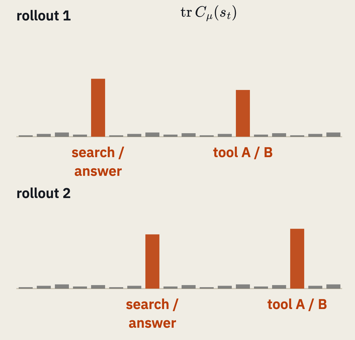
Two agent rollouts, one bar per position (an illustration). The bar is tr C_μ(s_t), the expected squared size of the backward signal at that prefix. It is near zero wherever the sampler is sure and large only at the forks: whether to search or answer, and which tool to call.

At the output layer the parameters are indexed by the vocabulary: an entry of the unembedding row of token $c$ moves the logit of $c$ alone, its token Fisher is $h_k^2\,\smu(c)(1-\smu(c))$, and the rows of tokens that never compete cannot move (Part 2, section 1). Every parameter below the unembedding reaches the logits through $h$, so $\kappa_{i,a}=w_a^\top u_i$, and its centered score at position $t$ is one vector pulled back through $u_i$:

The vector $\delta_t$ is the same for every parameter. Given the prefix, it has mean zero and covariance $C_\mu(s_t)$, and it is one of the centered output vectors, so it lies in the range of $C_\mu(s_t)$. Its expected squared size is a variance, at most the second moment about the most likely token’s vector $w_{a^\star}$; that token contributes zero and every other difference has norm at most $2B$:

Where the sampler is sure, the backward signal is nearly zero. Along a rollout it is flat except at forks, the few positions where several tokens compete, and at a fork with $n$ competitors it spans at most $n-1$ directions. A single draw can still be large: for a rare token $\|\delta_t\|$ can reach $2B$, and the bound holds on average over the draw.

2. The head’s update is low-rank, up to a leak

For a linear map that produces the unembedding input, the expected update splits into a part whose rank is set by the tokens that compete at forks, and a leak set by the sampler’s mass outside them.

← ▶ → 1 / 1

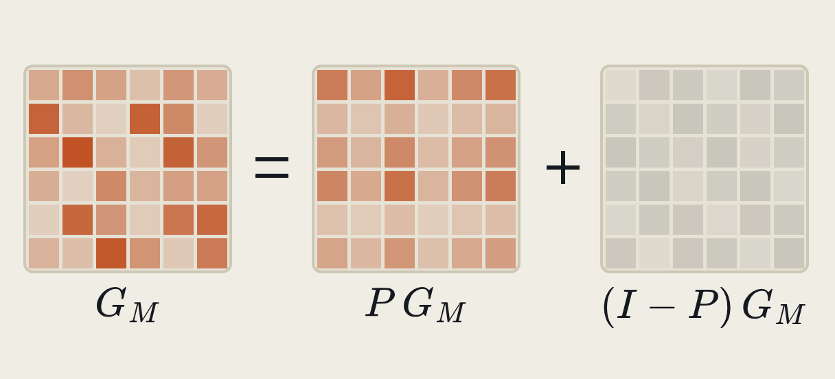
The head's expected update splits in two: PG_M, whose columns lie in the span D of differences between the competing tokens' output vectors, and a faint leak (I − P)G_M, set by the sampler's mass outside the competing tokens.

Let $M$ be a linear map with $h(s_t)=M x_t$, where the input $x_t$ is computed before $M$ and so does not depend on it. (In a transformer a final normalization sits between the last linear layer and the unembedding; section 4 adds it.) For every prefix $s$ choose a candidate set $K_s$ of tokens, and write

for the sampler’s mass outside the candidates and the span of differences of candidate output vectors, and $P$ for the orthogonal projector onto $D$. Then the expected update $G_M=\mathbb{E}_{\smu}\big[A\sum_t\delta_t x_t^\top\big]$ splits as $G_M=PG_M+(I-P)G_M$, with

The candidate sets are a free choice. At a fork, take the competing tokens. At a confident prefix, take the top token alone: one vector has no differences, so it adds no direction, and its leak $\rho_s=1-\max_a\smu(a\mid s)$ is small exactly there. Larger candidate sets lower the leak and raise the rank. The statement concerns the expected update at a fixed sampler; it makes no assumption about the inputs $x_t$ and needs no independence between the backward signal and the inputs.

3. What this says about LoRA

An adapter of rank $\dim D$ carries the head’s expected update up to the leak, and gradient descent on LoRA finds that subspace by itself.

Because $PG_M$ has rank at most $\dim D$, the best approximation of $G_M$ by a matrix of rank $r\ge\dim D$ is at least as good as $PG_M$ (Eckart & Young, 1936, in its easy direction):

with $U$ an orthonormal basis of $D$ and $V=G_M^\top U$. That is the shape of LoRA, an update $\Delta M=UV^\top$ (Hu et al., 2021, who write it $BA$). Here both factors have a meaning: $U$ is built from differences of the competing tokens’ output vectors, and $V$ records what the inputs look like at the forks.

LoRA reaches this subspace on its own. With the factor $U$ initialized at zero and $V$ at random, the first gradient on $U$ is $G_MV_0$, whose columns lie in the column space of $G_M$, inside $D$ up to the leak, while $V$ gets no gradient in that step.

How large $\dim D$ is depends on the task. When the forks are the same few decisions in rollout after rollout, with the same candidates, $D$ is small. For a broad task the union of competing tokens over all prompts can run into the thousands, and the bound grows with it. LoRA of rank one matches full fine-tuning in RL on math (Schulman & Thinking Machines Lab, 2025), so the useful part of the update can be much smaller than this count. Two further arguments explain that: the signal itself carries little, at most one bit per pass/fail episode (Information Bandwidth), and the Fisher weighs the directions unevenly (section 5).

4. Below the head

Below the head the same subspace is carried down along Jacobian paths; the final normalization adds one direction per position.

← ▶ → 1 / 1

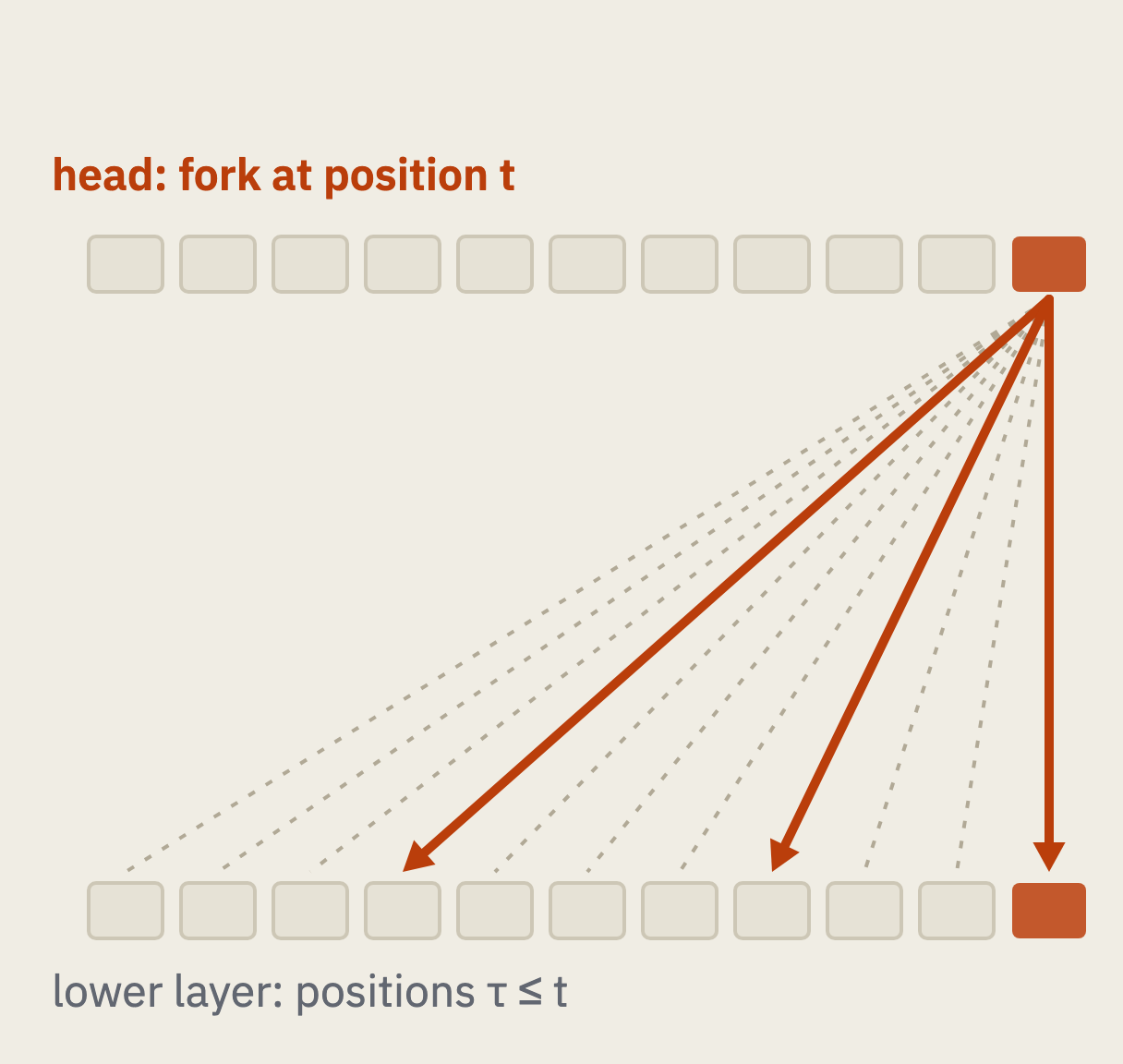
Below the head. A fork at position t (top row) reaches a lower layer (bottom row) at the positions τ ≤ t through the Jacobians J_t,τ. Thick arrows are the few strong paths, where attention looks; dashed lines are the weak ones.

For a matrix $M_\ell$ in a lower layer, write $o_\tau=M_\ell x_\tau$ for its output at position $\tau$ and $J_{t,\tau}=\partial h(s_t)/\partial o_\tau$ for the Jacobian that carries it to the last hidden state at a later position $t$. The gradient of the centered score sums over the earlier positions:

Each image $J_{t,\tau}^\top D$ has dimension at most $\dim D$, so the rank of the main part is at most $\dim D$ times the number of distinct maps $J_{t,\tau}^\top$ that carry signal. The bound is exact. The number of such maps is an empirical quantity; attention that concentrates on a few positions keeps it small.

In a transformer the last hidden state is a normalized residual stream, $h=g\odot r/\operatorname{rms}(r)$ with a learned gain $g$ (Zhang & Sennrich, 2019). With $\hat r=r/\|r\|$ and $\delta_t$ in $D$, as it is for the main part, the signal that reaches the residual stream at position $t$ is

the rescaled subspace, plus one direction per position, the position’s own residual direction, weighted by its overlap with the signal. Every layer adds its output to the residual stream, so the identity path hands this signal to the output of every layer; the Jacobians of attention and of the feed-forward blocks add the other paths.

5. The size of each coefficient gives LoRA’s shape

Counting directions gives a rank; weighing them by the Fisher shows where the update’s energy sits, and with a Kronecker-factored Fisher that place is a small block.

← ▶ → 3 / 3

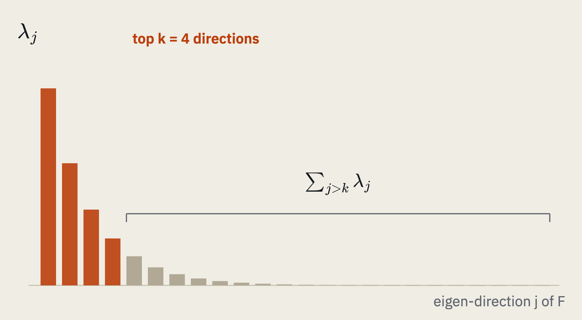
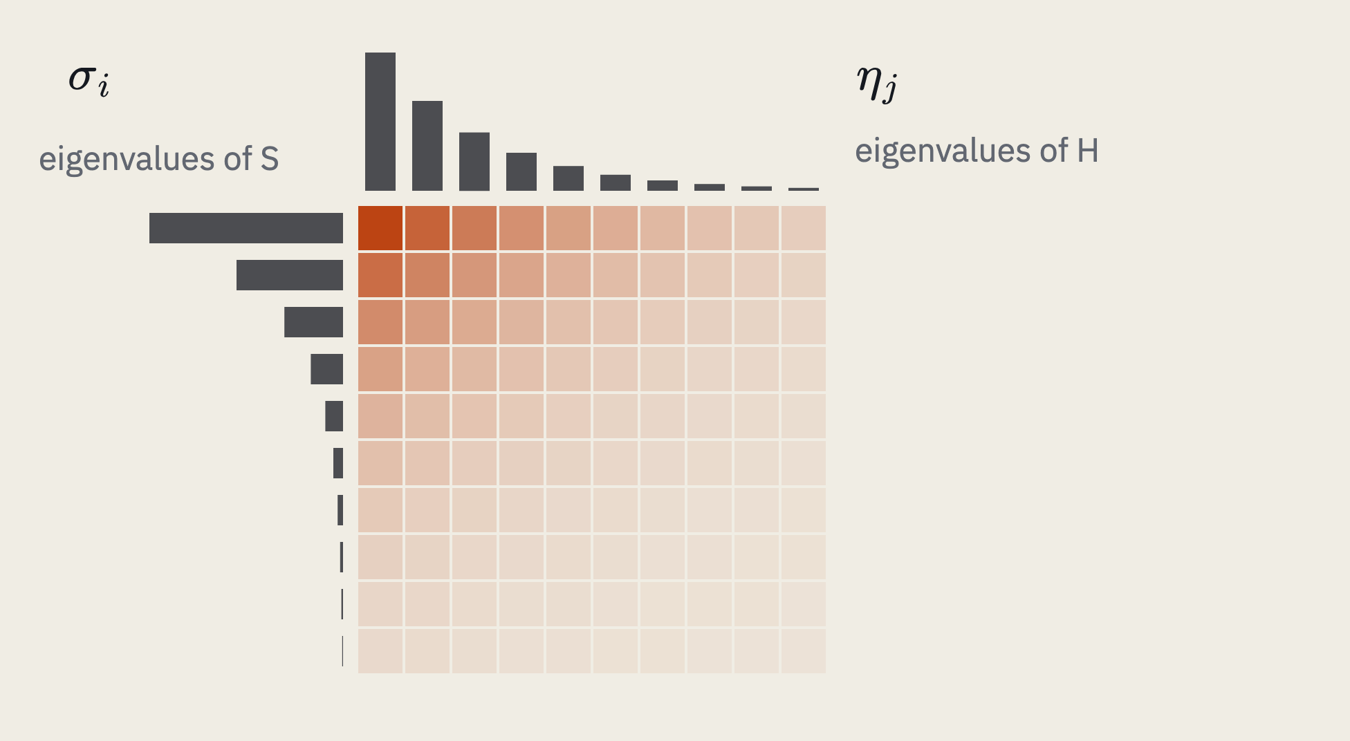
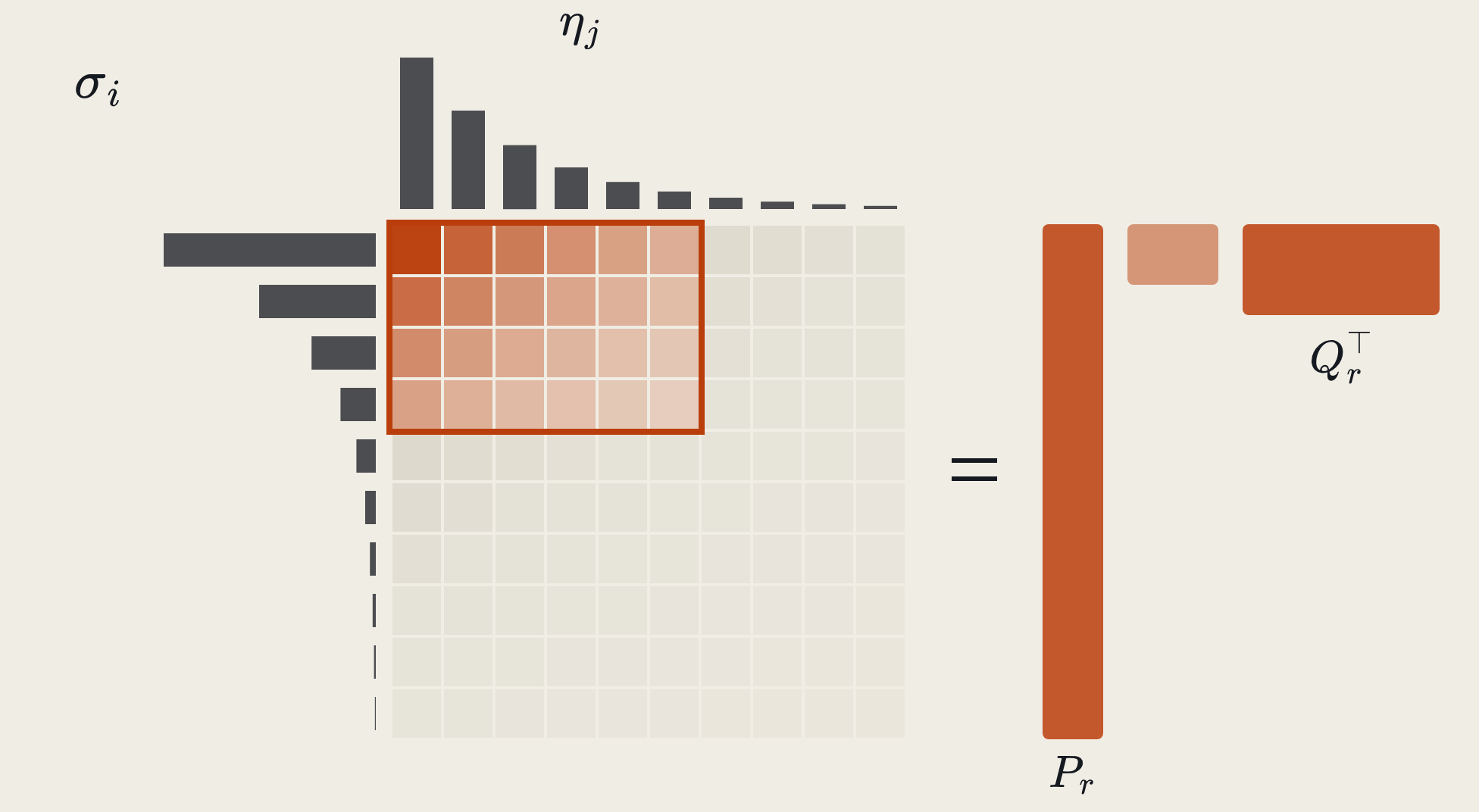
Capping each coefficient by std(A)·√(Tσ_iη_j) leaves a small top-left block, here four rows and six columns. In these bases the update is P_rΓQ_r^⊤: a tall factor, a small block Γ and a flat factor, which is LoRA's shape.

For any unit direction $w$ in parameter space, the Cauchy–Schwarz step of Part 1 gives $|w^\top G|\le\operatorname{std}_{\smu}(A)\sqrt{w^\top F^{\mu}w}$; the per-parameter cap is the case where $w$ is one coordinate. Along the eigenvectors $u_j$ of $F^{\mu}$, with eigenvalues $\lambda_j$, the coefficients are capped by $\sqrt{\lambda_j}$, and everything outside the top $k$ directions is bounded by the tail of the spectrum:

Take the head’s map $M$ of section 2, with input $x_t$ and backward signal $\delta_t$; its gradient at position $t$ is $\delta_t x_t^\top$. Cross terms between positions vanish as in the proof of section 2, so its Fisher is exactly $F_M=\mathbb{E}_{\smu}\sum_t(x_tx_t^\top)\otimes(\delta_t\delta_t^\top)$. The Kronecker-factored approximation, K-FAC (Martens & Grosse, 2015), treats $\delta$ and $x$ as independent and replaces each term by a product of averages over prefixes and positions. The Fisher then acts on a matrix $X$ from both sides, and its eigen-directions are outer products of the eigenvectors $p_i$ of $S$ and $q_j$ of $H$:

where the bars average over prefixes and positions, $T$ is the number of positions, and $\sigma_i$ and $\eta_j$ are the eigenvalues of $S$ and $H$. Lower layers fit the same form with their own backward signal, and there K-FAC is an approximation from the start. If $\sigma_i$ is small beyond the first $r_s$ and $\eta_j$ beyond the first $r_h$, every coefficient outside an $r_s\times r_h$ block is small, and in these bases the update is $G_M\approx P_r\,\Gamma\,Q_r^\top$, of rank at most $\min(r_s,r_h)$: a tall factor $P_r$ of the top eigenvectors of $S$, a small block $\Gamma$, and a flat factor $Q_r^\top$ of the top eigenvectors of $H$. The tall factor spans the output directions the layer is most sensitive to; the flat one spans the input directions it sees most.

At the head, $\mathbb{E}[\delta_t\delta_t^\top\mid s_t]=C_\mu(s_t)$, so $S$ is the average of the covariances of Part 2 along the rollouts, large only at forks. The two arguments meet there. Counting gives the rank bound of section 2 without any factorization; weighing explains why a rank far below that bound can suffice. At the unembedding itself the Kronecker form holds exactly at each prefix: its token Fisher is $\big(\operatorname{diag}(\smu)-\smu\smu^\top\big)\otimes hh^\top$ (Part 2, section 1).

6. What the measurements show

Accumulated updates have full numerical rank and still keep a large share of their energy in a few directions; the bounds above describe one expected step, and three things separate it from the accumulated change.

The measurements:

• Few coordinates, full numerical rank. RL changes 5–30% of the parameters, and the update to almost every matrix is nearly full rank (Mukherjee et al., 2025). Part of this sparsity is precision: a change too small to alter a bfloat16 weight does not register (Zhu et al., 2025).
• Full rank, concentrated energy. Across six runs of on-policy distillation, the median matrix has full numerical rank at a relative threshold of $10^{-5}$, while its top 16 singular values hold 20–41% of the energy and its stable rank is 7–20. Two RL runs with verifiable rewards look the same (top-16 energy 19.6% and 26.9%, stable rank 16.1 and 12.4); offline distillation, which trains on another model’s outputs, is diffuse (8.6% and 82.7) (Yu et al., 2026).
• The subspace forms early. Over training the stable rank of the cumulative update contracts for RL with verifiable rewards, stays in a narrow band for on-policy distillation, and expands for supervised fine-tuning (SFT); restricting on-policy distillation to the subspace of its early updates preserves its performance (Shen et al., 2026).
• Low capacity is enough. Rank-one LoRA matches full fine-tuning in RL (Schulman & Thinking Machines Lab, 2025).
• The optimizer shapes the support. With stochastic gradient descent (SGD), full fine-tuning in RL changes fewer than 0.02% of the parameters, more than 1,000 times fewer than with AdamW, and matches or beats its accuracy (Mukherjee et al., 2026).

What separates one expected step from the accumulated change:

• The optimizer. An SGD step is proportional to the gradient, so the cap of Part 1 and the subspace of section 2 apply to its expected step. Adam divides each entry by its own running scale, which is not a linear map on the matrix: its first step is close to the entrywise sign of the gradient, and the sign pattern of a matrix of rank two or more is generally full rank. Small coordinates are lifted toward the step size of large ones, which spreads the change over more coordinates and more directions.
• The forks move. As training sharpens the sampler, the competing tokens and their output vectors change, and so does $D$. The initial high-Fisher coordinates keep 70–78% of their membership over 1,000 steps (Zhang, Mukherjee & Peng, 2026), so the set of directions that the steps use grows over training.
• Noise and the leak fill every direction weakly. Numerical rank counts singular values above $10^{-5}$ of the largest, so a weak floor of noise makes any accumulated matrix full rank. Stable rank and energy fractions measure where the update’s weight lies, which is what the bounds describe.

7. Supervised fine-tuning leaves the forks

Without centering, the gradient of supervised fine-tuning points toward whichever token the data demonstrates, at every position where data and model disagree, so its directions add up position by position.

At prefix $s$, the gradient of the log-likelihood with respect to the unembedding input is $w_{y}-\bar w_p(s)$ for a demonstrated token $y$, where $\bar w_p$ is the model’s average output vector. Averaged over the data distribution $q$ it is a shift of the mean:

This is the mean shift of Part 2, section 3, read in hidden space. It is nonzero wherever the data disagrees with the model, including prefixes where the model is sure, and there it points from the model’s top token toward the demonstrated one, which need not be among the model’s candidates. Confident positions, which send almost nothing in on-policy policy gradient, contribute in full, and each contributes its own direction. The measurements agree: in a controlled comparison on Qwen3-8B, 8.1% of the weights are unchanged after SFT, against 51.6% after on-policy distillation and 77.2% after RL with verifiable rewards, counted at bfloat16 precision (Shen et al., 2026), and offline distillation has the most diffuse spectrum of the runs above (Yu et al., 2026). On-policy distillation samples from the model and centers its score the same way as RL, and it falls between the two.

8. Scope and open questions

• Where it is exact. For the unembedding input and for a linear map that produces it. Through the final normalization it picks up one direction per position; below that, the number of Jacobian paths that carry signal is measured.
• One step, first order. Every bound here is for the expected update at a fixed sampler. The forks drift during training, and a bound on the accumulated change would have to control that drift.
• The optimizer. For SGD the subspace argument applies to the expected step. For Adam it applies to the gradient, and the per-coordinate scaling raises both the rank and the support of the step.
• Temperature. At temperature one every token has positive probability, so formally the whole vocabulary competes at every prefix; the leak term absorbs the tail, and top-p sampling makes the candidate sets exact.
• What to measure. The spectrum of $S$, the average of $C_\mu(s_t)$ along real rollouts; the number of distinct forks per task; and the overlap between the top singular vectors of a measured head update and the span of differences of the competing tokens’ output vectors.

The series in one line. A score centered under the sampler makes the update a covariance capped by the Fisher (Part 1); that Fisher is concentrated when the sampler favors a few tokens that react alike, and without centering a mean shift escapes it (Part 2); a response moves only as far as it resembles what the sampler produces (Part 3); and the same competing tokens make the update sparse in the vocabulary and low-rank in hidden space (this part).

References

• Y. Zhang, S. Mukherjee, H. Peng. Understanding LLM Parameter Update Sparsity through the Lens of Fisher. arXiv, 2026.
• S. Mukherjee, L. Yuan, D. Hakkani-Tür, H. Peng. Reinforcement Learning Finetunes Small Subnetworks in Large Language Models. NeurIPS 2025.
• S. Mukherjee, L. Yuan, P. Jayasinha, D. Hakkani-Tür, H. Peng. Do We Need Adam? Surprisingly Strong and Sparse Reinforcement Learning with SGD in LLMs. arXiv, 2026.
• G. Yu, W. Liu, Y. Hu, et al. Dense Supervision, Sparse Updates: On the Sparsity and Geometry of On-Policy Distillation. arXiv, 2026.
• Z. Shen, Y. Li, Q. Yin, et al. On the Geometry of On-Policy Distillation. arXiv, 2026.
• H. Zhu, Z. Zhang, H. Huang, et al. The Path Not Taken: RLVR Provably Learns Off the Principals. arXiv, 2025.
• J. Schulman and Thinking Machines Lab. LoRA Without Regret. Thinking Machines Lab: Connectionism, 2025.
• E. J. Hu, Y. Shen, P. Wallis, et al. LoRA: Low-Rank Adaptation of Large Language Models. ICLR 2022.
• J. Martens, R. Grosse. Optimizing Neural Networks with Kronecker-factored Approximate Curvature. ICML 2015.
• C. Eckart, G. Young. The Approximation of One Matrix by Another of Lower Rank. Psychometrika, 1936.
• B. Zhang, R. Sennrich. Root Mean Square Layer Normalization. NeurIPS 2019.
• Y. Li. Information Bandwidth in Reinforcement Learning. Blog, 2025.

Citation

@online{li-2026-low-rank-hidden-space,
  title  = {Sparse in the Vocabulary, Low-Rank in Hidden Space},
  author = {Li, Yingru},
  year   = {2026},
  month  = oct,
  url    = {https://richardli.xyz/post/low-rank-hidden-space/}
}