Around the Sampler: Tangent, Remainder and KL
Off-Policy RL at Scale, Part 1: an exact first-order view of the off-policy update, with a sequence-level bound and no horizon factor
Off-Policy RL at Scale · Part 1 of 2. Part 2 keeps the gap fixed as the run grows. This builds on When Speed Kills Stability, Trust Region Masking, the Optimal Token Baseline and Beyond Precision.
- Measured from the sampler, the gain of any update is exactly a tangent plus a remainder.
- The tangent is a covariance loss: its gradient needs only the trainer.
- The remainder is at most Rmax · KLseq. The bound is for the whole sequence, with no horizon factor.
- Score centering, per-token importance sampling, a KL pull and a sequence mask all fall out of this picture, and methods differ by one coefficient, β.
The figures step through like slides. Use → or ▶, and step back with ←.
1. One off-policy gap
Every token is drawn by one policy and trained through another.
One off-policy gap, whatever its source: numerics and age together.
The levers that buy throughput (fast kernels, asynchrony, larger batches) open a gap between $\ps$, which drew the token, and $\pt$, which takes the gradient. The gap has two sources: engine mismatch, which is present even at identical weights, and staleness. Part 2 models both. The gap sets the bias of the update, the batch sets its variance, and the step size multiplies both:
one reward × thousands of token gradients
This post is about the bias: what the update should be when the data came from $\ps$. From here on, $\mathbb{E}$ and $\mathrm{Cov}$ are over rollouts drawn by the sampler.
2. Gain = tangent + remainder
Measured from the sampler, the gain of an update is exactly a tangent plus a remainder.
The best step
Never worse than the sampler.
A KL budget replaces R max by R max + λ: a smaller step in the same direction.
With $\ell_t = \log\frac{\pt(y_t)}{\ps(y_t)}$ and $\ell = \sum_t \ell_t$, reweighting whole rollouts gives the gain exactly:
$$ \text{gain} = J(\pt) - J(\ps) = \mathbb{E}\big[R\,(e^{\ell}-1)\big]. $$At each prefix, the mean of $\ell_t$ under the sampler is $-\mathrm{KL}_t$. So $\ell$ splits into a centered first-order sum minus a second-order sum of token KLs. The first-order part gives the tangent:
$$ \text{tangent} = \mathrm{Cov}\Big(R,\ \sum_t \big(\ell_t-\bar\ell_t\big)\Big) = \sum_t \mathrm{Cov}\Big(R,\ \log\pt(y_t) - \mathbb{E}_{\ps}\big[\log\pt\big]\Big) + C . $$This is the covariance loss. Computing its value needs the ratio, but its gradient needs only the trainer. Whatever the tangent misses is the remainder, and that remainder is the bias:
$$ \text{remainder} = \mathbb{E}\big[R\,(e^{\ell}-1-\ell)\big] - \mathbb{E}\Big[R\sum_t \mathrm{KL}_t\Big]. $$The bound, in three facts.
- Both weights are non-negative.
- Both have the same mean, $\mathbb{E}[e^{\ell}-1-\ell] = \mathbb{E}[\sum_t \mathrm{KL}_t] = \mathrm{KL}_{\text{seq}}$.
- The reward lies in $[0, R_{\max}]$.
So each expectation lies in $[0, R_{\max}\mathrm{KL}_{\text{seq}}]$, and therefore
$$ \boxed{\ \big|\text{remainder}\big| \le R_{\max}\,\mathrm{KL}_{\text{seq}}\ } $$The bound holds at any distance from the sampler and has no horizon factor. Per-position trust-region bounds are governed by the worst token instead. For a 4,096-token rollout with worst-token KL $10^{-4}$, sequence KL 0.01 and reward scale 1:
| Bound on the surrogate error | Form | Value |
|---|---|---|
| Classical (TRPO) | $T(T-1)\,D_{\mathrm{KL}}^{\text{tok,max}}$ | 1677 |
| Mixed (TRM) | $2T\sqrt{D_{\mathrm{KL}}^{\text{tok,max}}\,\mathrm{KL}_{\text{seq}}}$ | 8.2 |
| Sequence-level (this post) | $R_{\max}\,\mathrm{KL}_{\text{seq}}$ | 0.01 |
For very long rollouts the sequence KL can exceed one, and then no bound that ignores the reward certifies anything. I use the bound for the shape of a good step, not as a certificate.
To second order, the remainder is a reward-weighted quadratic
$$ \text{remainder} \approx \tfrac12\,\mathrm{Cov}\Big(R,\ \big(\textstyle\sum_t c_t\big)^2 - \sum_t V_t\Big), \qquad c_t = \ell_t - \mathbb{E}_{\ps}[\ell_t], \quad V_t = \mathrm{Var}_{\ps}(c_t). $$The $c_t$ are martingale differences, so their cross terms vanish in expectation. That is why the quadratic has mean zero and appears as a covariance. Its sign is not fixed, and its scale is the sequence KL, since $\mathrm{KL}_{\text{seq}} \approx \tfrac12\sum_t \mathbb{E}[V_t]$.
3. The best step
The lower edge of the band has a closed-form top, and it is never worse than the sampler.
The last frame of the figure above shows the lower bound $\text{gain} \ge \text{tangent} - R_{\max}\mathrm{KL}_{\text{seq}}$. It is concave in the trainer’s logits and zero at the sampler. Its maximizer reweights the sampler at every prefix by one plus the advantage $A$ over $R_{\max}$:
$$ \pi^\star = \ps\cdot\Big(1 + \frac{A}{R_{\max}}\Big). $$Since the bound is zero at the sampler, this step is never worse than the sampler. Among the changes a network can make, the natural-gradient step comes closest to it. A KL budget with multiplier $\lambda$ replaces $R_{\max}$ by $R_{\max}+\lambda$: a smaller step in the same direction.
Why, in the one-token case
The bound equals $\sum_y \ps(y)\big(A(y)+R_{\max}\big)\log\pt(y)$ plus a constant. It is maximized by $\pt \propto \ps\,(A+R_{\max})$, which already sums to one because $\sum_y \ps A = 0$.
4. Score centering
The gradient of the tangent raises the drawn token and lowers every token by how often the sampler draws it.
Averaged over what the sampler draws, it is zero: a constant reward moves nothing.
Averaged over what the sampler draws, the raises and lowerings cancel, so a constant reward moves nothing. The plain score averages to zero under the trainer, not under the sampler, so without centering even a constant reward pushes the policy. That is the off-policy bias in its simplest form. Score centering has an independent public treatment in Marek & Ryabinin (2026); here it is simply the gradient of the tangent.
5. Per-token importance sampling: same tangent, more variance
PPO and GRPO multiply by a ratio where the covariance loss subtracts a mean, and multiplication costs variance.
width: how often the token is drawn
height: its ratio
ratio 1
a rare token
The ratio averages to 1. But a token the sampler rarely draws and the trainer prefers gets a large one, and the estimate jumps whenever it appears: E[r²] = 1 + χ², far above the KL.
At the sampler it has the same tangent, so to first order it takes the same step. But a token that the sampler rarely draws and the trainer now prefers gets a large ratio, and the estimate jumps whenever that token appears. The $\chi^2$ divergence, which is dominated by such tokens, can be far above the KL, and the KL is all the bound controls. Clipping tames the jumps, but gives up first-order correctness on exactly those tokens.
6. One knob: how hard to pull toward the sampler
Every method is the tangent plus some multiple $\beta$ of a pull toward the sampler.
- Pull. Add $\beta\,\mathrm{KL}_{\text{seq}}$ to the loss. Its gradient is the mean score, which points toward the sampler and ignores the reward. The sequence KL is a divergence between the state distributions of the two policies (the state is the prefix), as in Divergence-Augmented Policy Optimization (NeurIPS 2019).
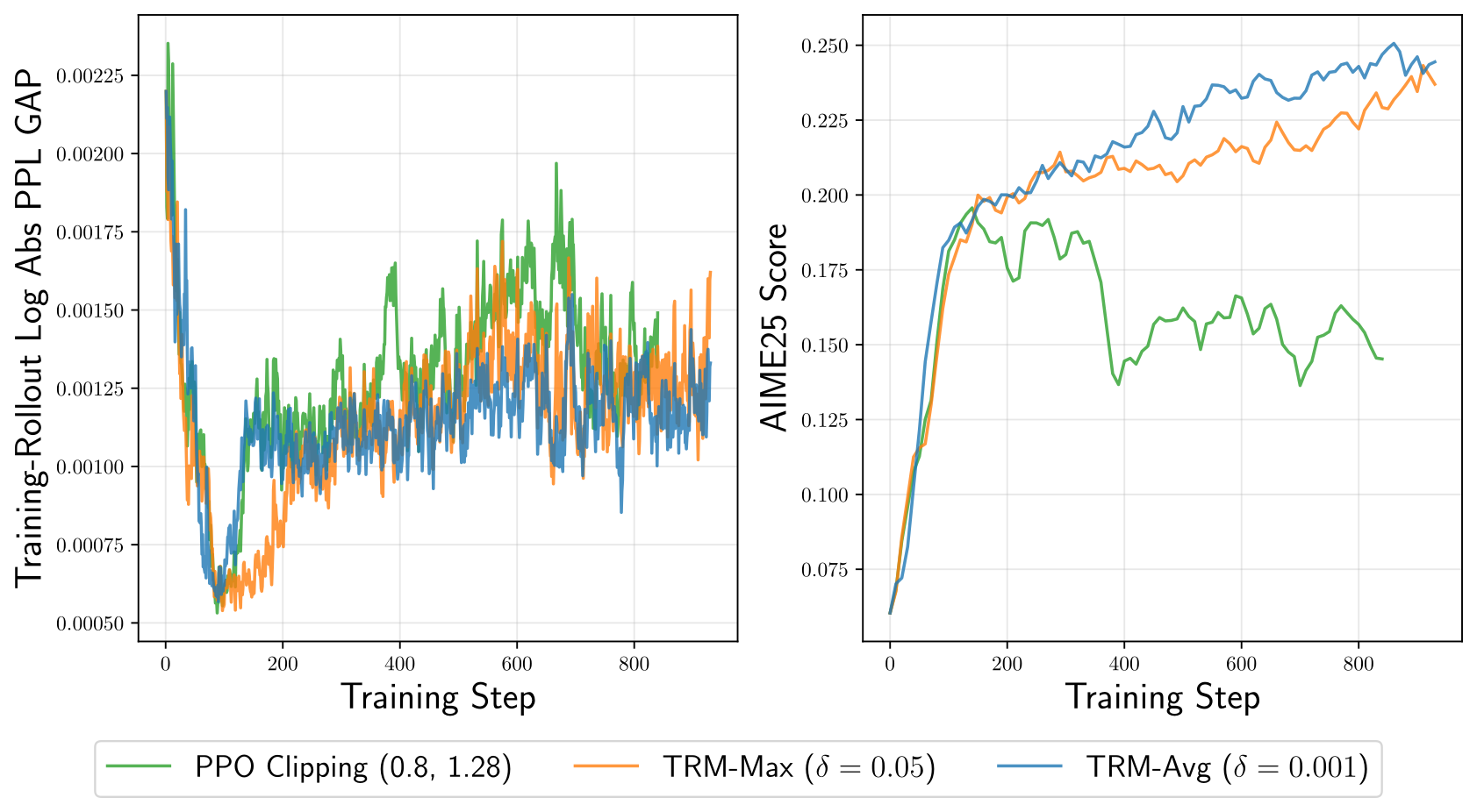
- Reject. Drop a rollout whose sequence KL is too large, using $M(y) = \mathbf{1}[\sum_t \mathrm{KL}_t \le \tau]$. This is Trust Region Masking, which ships in veRL. Inside the mask the estimator is still first-order correct. The threshold must sit above the engine-mismatch floor.
| Method | Coefficient $\beta$ | What it does |
|---|---|---|
| Plain policy gradient | $R-b$, per rollout | An uncontrolled pull: toward the sampler on good rollouts, away from it on bad ones |
| Covariance loss, or unclipped ratios | $0$ | The tangent alone |
| Certified lower bound | $R_{\max}$ | As large as the true correction can be, and blind to the reward |
| With a KL budget | $R_{\max}+\lambda$ | A smaller step in the same direction |
$\beta$ is a stability–plasticity knob: it sets how much the learner trusts where its data came from. How $\beta$, the step size and the queue should move as the run grows is the subject of Part 2.
References
- J. Liu, Y. Li, et al. When Speed Kills Stability: Demystifying RL Collapse from the Training-Inference Mismatch. Blog, 2025.
- Y. Li, J. Liu, et al. Trust Region Masking for Long-Horizon LLM Reinforcement Learning. ICML 2026.
- Q. Wang, Y. Li, J. Xiong, T. Zhang. Divergence-Augmented Policy Optimization. NeurIPS 2019.
- M. Marek, M. Ryabinin. Score Centering Stabilizes Off-policy Reinforcement Learning. arXiv, 2026.
- J. Schulman, S. Levine, P. Abbeel, M. Jordan, P. Moritz. Trust Region Policy Optimization. ICML 2015.
Citation
@online{li-2026-around-the-sampler,
  title  = {Around the Sampler: Tangent, Remainder and KL},
  author = {Li, Yingru},
  year   = {2026},
  month  = oct,
  url    = {https://richardli.xyz/post/offpolicy-around-the-sampler/}
}

Yingru Li
Member of Technical Staff
Core contributor to RL fundamentals at xAI (now SpaceX Super Intelligence); I make reinforcement learning on frontier models stable, efficient, and scalable.